

Building upon the previous tutorial on one-hot encoding, this tutorial will explore the concept of word embeddings and implement this with real-world data.
For our example, we extract patient summaries from PubMed and label those that had COVID-19 vs. not COVID-19. Word embeddings are created from text, and the embeddings are trained as part of a neural network to perform a classification task. Through training, the computer will learn word relationships.
Pre-requisites:
- Basic knowledge of neural networks
- Azure Data Studio
- Docker
- Python 3.10.3
- SQL Server on Mac (on-prem)
All resources can be found here.
A short intro to Word Embeddings
Word Embeddings were a bit of a complex concept to grasp, until I got into the weeds of building one. I’ve come to appreciate that they are an important concept in deep learning, for the reason that word meanings can be approximated mathematically.
To best understand the intuition behind word embeddings, I highly recommend reading this blog post from Christopher Olah.
There are a number of techniques available to build a word embedding, including using pre-trained embeddings generated by GloVe, word2vec, etc. In this tutorial, we will build an embedding from scratch.
Let’s get data
I selected a dataset of ~167K PubMed patient summaries via HuggingFace. The data is loaded into SQL Server on a Mac.
Start SQL Server via the terminal, giving the username and password:
1
$ mssql -u <sql server username> -p <sql server password>
Connect SQL Server to Azure Data Studio to query the data.
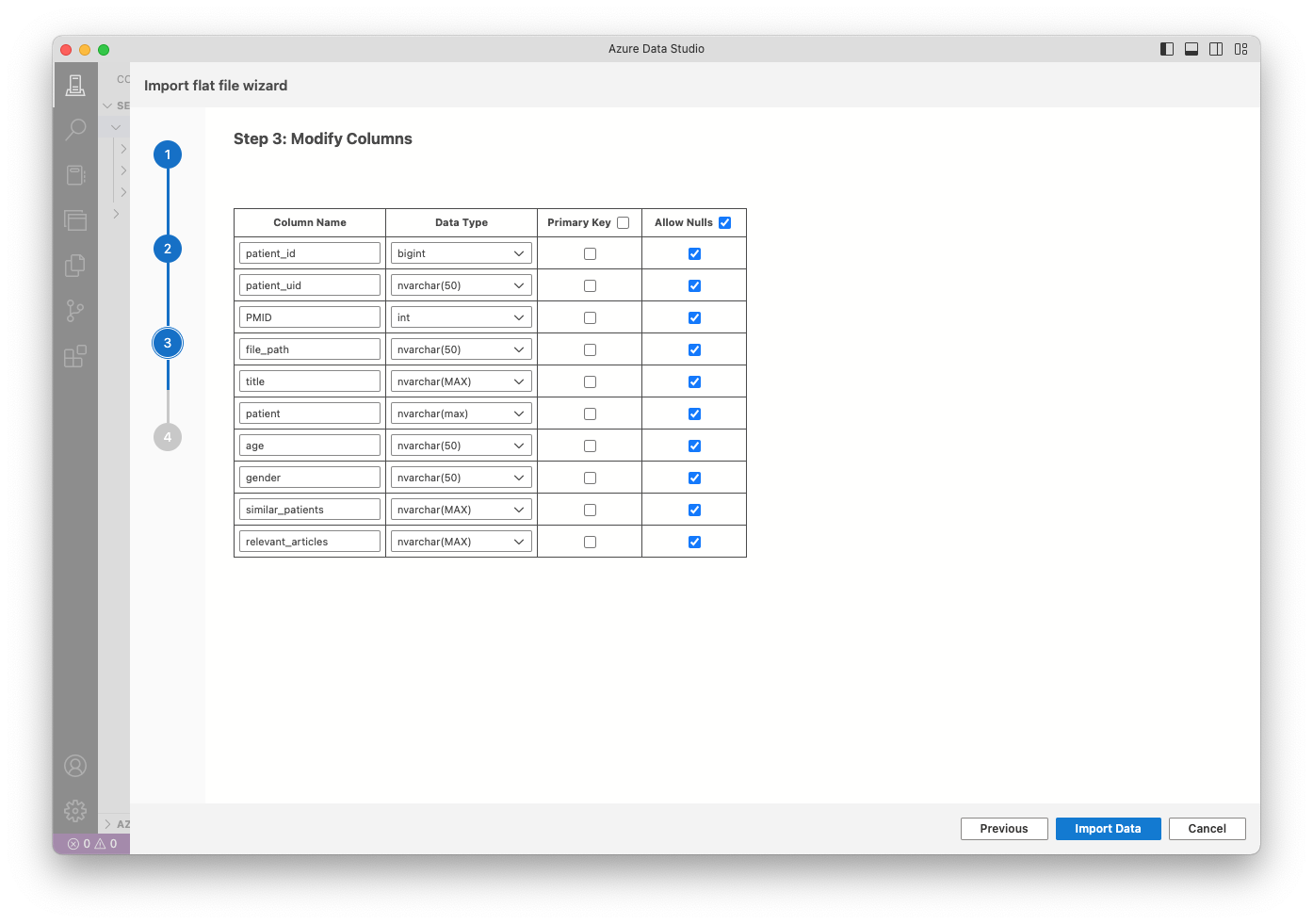
Attached is a screenshot to modify the columns before importing the data:
Run the below query to return the first 100 records and save as csv.
1
2
3
4
5
6
7
8
9
10
11
SELECT TOP (100) [patient_id]
  ,[patient_uid]
  ,[PMID]
  ,[file_path]
  ,[title]
  ,[patient]
  ,[age]
  ,[gender]
  ,[similar_patients]
  ,[relevant_articles]
FROM [test].[dbo].[PMC-Patients]
Define class labels
Since this is a binary classification task, we will label the dataset as:
- patients with COVID-19 = ‘1’
- patients without COVID-19 = ‘0’
1
2
3
4
5
6
7
8
9
10
11
12
13
14
15
labels = []

df['label'] = ''

for index, row in df.iterrows():
    if 'COVID-19' in row['patient']:
        row['label'] = '1'
    else:
        row['label'] = '0'

    labels.append(row['label'])

labels_arr = np.array(labels).astype(float)

print(labels_arr)
1
2
3
4
5
[1. 0. 0. 0. 0. 0. 0. 0. 1. 1. 1. 0. 0. 0. 1. 0. 0. 0. 0. 0. 0. 1. 1. 0.
 0. 0. 0. 0. 0. 0. 0. 0. 0. 0. 0. 0. 0. 0. 0. 0. 0. 1. 0. 0. 0. 0. 0. 0.
 0. 0. 0. 0. 0. 0. 0. 0. 0. 0. 0. 0. 0. 0. 0. 0. 0. 0. 0. 0. 0. 0. 0. 0.
 0. 0. 0. 0. 0. 0. 0. 0. 0. 0. 0. 0. 0. 0. 0. 0. 0. 0. 0. 0. 0. 1. 1. 0.
 0. 0. 1. 0.]
Create a corpus
Now that we have our labeled dataset, we create a corpus. We take the 1st sentence from each document. A sample of the first 3 documents is below:
1
2
3
4
['This 60-year-old male was hospitalized due to moderate ARDS from COVID-19 with symptoms of fever, dry cough, and dyspnea.',
'We describe the case of a 55-year-old male who presented to the emergency department via emergency medical services for the chief complaint of sudden onset shortness of breath that woke him from his sleep just prior to arrival.',
'A 20-year-old Caucasian male (1.75 m tall and 76 kg (BMI 24.8)), was admitted to the medical department for persistent hyperpyrexia, severe sore throat, dyspnea, and impaired consciousness with stupor.,
...]
For 100 documents, there are 2541 total words in the corpus.
Convert text to integers
Since we saw the limitations with one-hot encoding, a better approach would be to assign each word a unique integer. The integer encoding for a specific word remains the same across all documents, so this will reduce the size of the corpus to unique words.
To do this, Keras provides a handy Tokenizer() API that can handle multiple documents. For a deeper understanding of its implementation, see this tutorial.
1
2
3
4
5
6
7
8
9
10
11
12
13
14
15
16
17
18
# integer encode words per document
encod_corp = []

# fit tokenizer on docs
t = Tokenizer(filters='!"#$%&()*+,/:;<=>?@[\\]^_`{|}~\t\n')
t.fit_on_texts(corp)
encod_corp = t.texts_to_sequences(corp)

# get unique words
vocab = t.word_index

# print vocab list
print("vocab:")
for i,v in enumerate(vocab, 1):
   print(i,v)

vocab_size = len(vocab)
print('Vocab size = %s unique words' % vocab_size)
1
2
3
4
5
6
7
8
vocab:
1 a
2 of
3 with
4 and
5 the

Vocab size = 931 unique words
Out of 2541 total words, 931 unique words are found.
Pad the documents
Keras requires that all documents must be the same length. We find the maximum length of a document, which is 55 words. Zeroes are then added to the shorter documents using the pad_sequences function:
1
2
3
4
# pad the documents with zeros
pad_corp=pad_sequences(encod_corp,maxlen=maxlen,padding='post',value=0.0)

print(pad_corp)
1
2
3
4
5
[[ 31 281  10   7 160  44   6 282 283  28  54   3  84   2  29  45  36   4
  161   0   0   0   0   0   0   0   0   0   0   0   0   0   0   0   0   0
    0   0   0   0   0   0   0   0   0   0   0   0   0   0   0   0   0   0
    0]
   ...
The above array represents the text of Document 1.
Create an embedding
To create the embedding, we create a Keras Sequential model. Sequential means that each layer in the network has exactly one input and one output. To define the embedding, we need 3 inputs:
- input_dim: size of vocabulary
- output_dim: embedding dimension
- input_length: maximum length of a document
A output_dim = 2 means that every vocabulary word is represented by a vector that contains 2 elements, or features. These numbers can be chosen arbitrarily. A larger output_dim will have more features to train on, but will also be more computationally expensive.
Once the embedding layer is added to the network, the learning process is configured, and we run model.predict() to generate the predicted outputs.
We can also add other hidden layers (Flatten, Dense) to discover more complex patterns in the data. These will be discussed once we train the embeddings.
1
2
3
4
5
6
7
8
9
10
11
12
13
14
15
16
17
18
19
20
21
22
# create keras model
model = Sequential()

# define embedding
embedding_layer = Embedding(
                        input_dim=vocab_size+1,
                        output_dim=2,
                        input_length=maxlen)

# add layers
model.add(embedding_layer)
model.add(Flatten())
model.add(Dense(1, activation='sigmoid'))

# configure the learning process
model.compile(
        optimizer='adam',
        loss='categorical_crossentropy',
        metrics=['accuracy'])

# model prediction
embedding_output = model.predict(pad_corp)
Visualize intial embeddings
The embedding layer is a lookup table, which represents each word as floating point values (weights) in the dimension specified. These weights are initialized randomly before training the model. The weights can be obtained as follows:
1
2
3
4
5
6
# embedding layer
embedding_layer = model.get_layer(index=0)

embedding_layer_weights = embedding_layer.get_weights()[0]

print(embedding_layer_weights)
Since the output_dim = 2, the embedding_layer_weights consists of each word represented by 2 weights:
1
2
3
4
5
6
7
8
9
10
[[ 7.04301521e-03  3.39607336e-02] (index 0)
 [ 4.43325080e-02 -4.35174219e-02] --> 'a'
 [-1.84080116e-02 -4.48269024e-02] --> 'of'
 [-4.74609025e-02  4.29279730e-03] --> 'with'
 [ 1.24161355e-02  4.76875566e-02] --> 'and'
 [-1.89721715e-02 -2.00293791e-02] --> 'the'
 [-2.18192935e-02 -4.75601330e-02] --> 'to'
 [-2.51929164e-02 -9.96438414e-03] --> 'was'
...]]
The embedding_output is the result of the embedding layer for a given input sequence. For Document 1, we see that each value from the embedding layer is mapped to a word in that document:
1
2
3
4
5
6
7
8
[[[ 2.08440907e-02  3.52325179e-02] --> 'This'
  [-1.70833841e-02 -4.37318459e-02] --> '60-year-old'
  [-4.54872735e-02  1.42193772e-02] --> 'male'
  [-2.51929164e-02 -9.96438414e-03] --> 'was'
  [-4.34226505e-02 -2.67695189e-02] --> 'hospitalized'
  [-3.18809636e-02  3.46260779e-02] --> 'due'
  [-2.18192935e-02 -4.75601330e-02] --> 'to'
  ...]]]
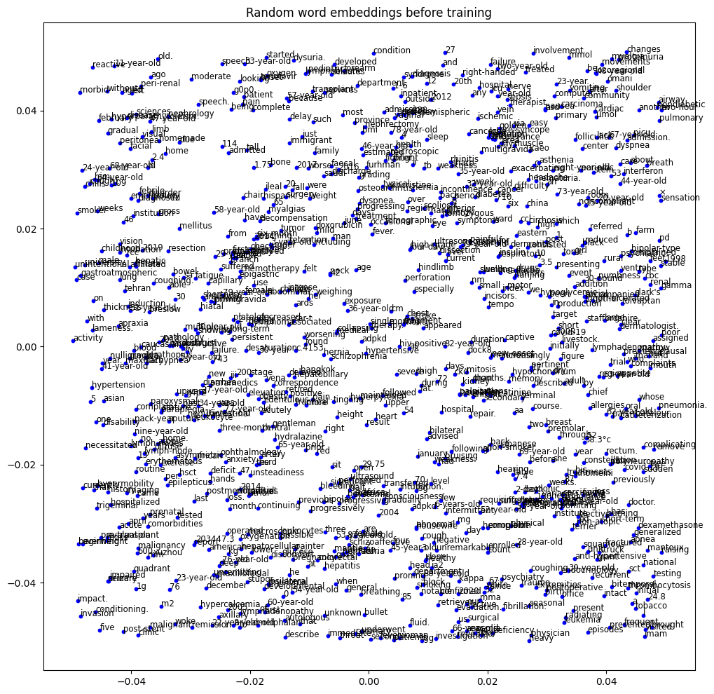
Let’s see how this looks visually. Since these embeddings are not trained, it would make sense that the words are fairly scattered:
Visualize trained embeddings
After adding the embedding layer, we have a 55 x 2 (doc length x embedding dimension) matrix. We need to compress (flatten) this into a 1D vector, to send to the next hidden (dense) layer.
As shown above, we add the Flatten and Dense layers to the model.
Summary of layers:
1
2
3
4
5
6
7
8
9
10
11
12
13
14
_________________________________________________________________
 Layer (type)                Output Shape              Param #
=================================================================
 embedding_28 (Embedding)    (None, 55, 2)             1864

 flatten_17 (Flatten)        (None, 110)               0

 dense_17 (Dense)            (None, 1)                 111

=================================================================
Total params: 1975 (7.71 KB)
Trainable params: 1975 (7.71 KB)
Non-trainable params: 0 (0.00 Byte)
_________________________________________________________________
The 55×2 matrix is now reduced to a 110-element vector by the Flatten layer.
Finally, we train the model on the classification task and evaluate its performance.
1
2
# fit the model
model.fit(pad_corp, labels_arr, epochs=50, verbose=1)
1
2
3
# evaluate the model
loss, accuracy = model.evaluate(pad_corp, labels_arr, verbose=1)
print('Accuracy: %f' % (accuracy*100))
1
2
4/4 [==============================] - 0s 2ms/step - loss: 0.0000e+00 - accuracy: 0.8900
Accuracy: 88.999999
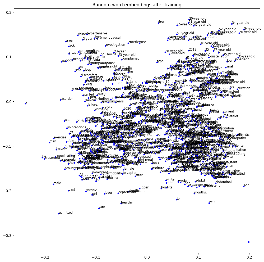
Since these embeddings are now trained, we can visualize more defined clusters with ~89% accuracy for the prediction task.
Conclusion
In this tutorial, we explored how to create word embeddings from scratch, using a neural network to perform a classification task. By taking sample text from PubMed patient summaries, we were able to train a neural network to classify patients who had COVID-19 and those that did not. In doing so, we were also able to train the embeddings, such that words with similar meanings were visually placed closer together.
We can boost the performance of the training accuracy by adding in a different layer, such as a convolution layer. I will explore this in a future post.
References
- http://colah.github.io/posts/2014-07-NLP-RNNs-Representations
- https://huggingface.co/datasets/zhengyun21/PMC-Patients/tree/main
- https://builtin.com/software-engineering-perspectives/sql-server-management-studio-mac
- https://www.sqlshack.com/sql-server-data-import-using-azure-data-studio/
- https://keras.io/
- https://machinelearningmastery.com/prepare-text-data-deep-learning-keras
- https://machinelearningmastery.com/use-word-embedding-layers-deep-learning-keras
- https://cs229.stanford.edu/summer2020/cs229-notes-deep_learning.pdf
- https://github.com/keras-team/keras/issues/3110